DayBRIGHT: Proposal + Test Video

The idea behind the DayBRIGHT project is to be able to visualize data through HDR light probes being influenced by various types of datasets. Each dataset, be it an RSS weather forecast, webcam frame sequence, arbitrary color selection, or any other value - will be translated into a common format to be applied to a core HDR image.

The DayBRIGHT project will be encapsulated within a core software application which will communicate with various data feeds. As mentioned, each type of data will be converted to a common format: a color gradient. A color gradient will allow for analysis of RGBA, as well as time by sampling across its length. Depth can also be calculated by converting RGBA to luminance values.

To render the results, the initial solution will be to use 3Delight, an implementation of the Renderman standard, first introduced by Pixar. Using Renderman will allow for programming flexibility and high-quality renders at HD resolutions, if needed. An example of the early results is shown below, where an orange -> cyan color gradient has been applied:

DayBRIGHT: Gradient Sampling

One of the core concepts of the DayBRIGHT project that I am developing over this semester is to enable the ability to drive HDR lighting over time using a variety of methods - the first of which is using a simple color gradient.

For every frame to be rendered, a copy of the core HDR image is created, then a color overlay operation is applied to that copy - with the color applied being the current sample value of the gradient. This relationship is graphically represented below:


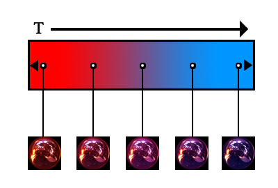
Fig 1.1: Graphical example of gradient sampling applied to image

Mind.Scribble.Form

My mind blurred, sketched, articulated, and scribbled on paper - most of which makes little to no sense to me currently. I normally never write things down to remember for the future - I generally only do so to calculate or brainstorm on the spot. Apparently, in parallel with my messy drawings, I also take photos without much care either. I think I'll write that off as part of my "creative process" and hope that you believe me (which you shouldn't).

Blast Radius

Several layers of particles revolving around a central sphere - each layer being rotated based on assigned attraction forces. Particles are symbolic of populous movement combined with the effect of unseen influence over collective entities - physically, socially, and otherwise.


Fig. 1.1: Straight-on shot


Fig 1.2: Corner angle


Source:
BlastRadiusMain.java
GLSL.java

Interactive and Time-Based HDR

I have been thinking a lot about pixels lately - most likely due to having a class with the given root word in it... twice. So, we have all of this information nicely packed within a frame - now what to do with it?

What I find interesting is how an image can be mined for data that is unseen upon first glance - and one of my favorite ideas in regard to this way of thinking is the creation and use of HDR images. High-Dynamic Range images are useful for an assortment of reasons - in the field of computer graphics, they are many times used as a light source. Paul Debevec is known as one of the groundbreaking researchers on the topic - and what initially began as technique for expensive high-end rendering has now been implemented in real-time in the past couple of years. Check out his site to see some of the amazing things HDR images can be used for.


Fig 1.1: Example of a light-probe HDR image
Credit: http://www.debevec.org


So, what else can been done with HDR - and how can it be used to create something interesting? For me, I want to explore moving away from leaving HDR lighting as a static image - and instead have it evolve over time while lighting a static scene. A few ideas are: time-lapse HDR lighting, real-time interaction with the HDR image itself, tying HDR colorization with weather forecasting, integration with existing data sets, and so forth.

Programming, Ubiquity, Devices, and You

After telling fellow students at ITP about the classes I decided to sign up for the coming Spring semester, I have often been asked the following two questions:

1. "Why are you taking programming centric classes if that is already one of your strengths?"

2. "Why aren't you taking any physical computer related classes?"

The answer to the first one is rather concise; I feel that staying constantly involved in software and mathematics allows me to build myself as a better overall problem-solver on both an analytical and creative basis. Writing code to solve a problem is concurrently a step-by-step breakdown of the problem itself; patterns emerge and reveal themselves, woven with systems of varying elegance and complexity. Understanding concepts which reveal such harmony will endure far past simply designing the next iPhone - leading me to the answer to the second question:

My position on physical computing at it pertains to projects at ITP (and in general) is that the development of devices which we physically interact with is inevitably obsolete. This is the century of biology - and consequently, biological micro-interfacing will be the future of device technology. Increased ubiquity leading to result/reward has nearly always been the trend in tool advancements - computing is to exist behind a curtain whenever possible. While it is certainly a valid venture to develop large-scale projects involving common electronics and so forth - I personally have little interest in pursuing similar implementation methods.

Software for Physical Display Project

Group: William McDonald, Sunghun Kim, Matt Parker

Further documentation:
Sunghun with videos / images
Matt on construction / mechanics

For our group project, we wanted to develop a physical system to represent graphical depth data. We decided to use a collection of sine and noise waves to start off with - as using depth data really only makes (practical) sense with a 3D grid.

Using Processing, a straight-forward GUI was created featuring four buttons, with a graphical representation of the waves being dynamically created to the right of the buttons. The fourth button allows the user to paint his/her own wave (or any shape, for that matter) and the software will generate a visualization and physical output for the image painted.



Fig 1.1: Drawing canvas allows user to draw images to physically visualize



Fig. 1.2: Visualization of user input wave drawing


To sample each wave - an algorithm was written which samples across the width of a given image proportional to the resolution of the physical system - in our case, 20 samples. At each sample - the program checks to see how far down (Y) the image it takes in pixels before a color other than white is found. Upon finding a color, the value of that sample is received by the simple equation of :

sample_value = y_coord / (image_height / max_value)




Fig 1.3: Graphical representation of sampling method on wave images


In regard to feeding this data into the servo motor array - we decided to use four arduino microprocessors connected via USB to the computer running the software application; with each arduino effectively controlling five servos:



Fig 1.4: Computer / Arduino / Servo array configuration

Shiver - Final

Fig 1.1: Splash screen for Shiver

The last week of work on Shiver has primarily been a focus on adding features on the GUI side and tying up some loose ends. The largest new feature is the ability to 'simulate' - which allows a user to simulate a full rotation (or however many wanted) of the globe, outputting the frames as an image sequence. This process allows the user to see the rotation as a movie clip running at full speed. The video in this blog entry is derived from that process.



Fig 1.2: Simulate options window


Shiver is still very much a work in progress - however, I am pleased with the result of my work over the past 6-7 weeks, particularly with knowing that I was able to achieve high-quality imagery in real-time using Python and OpenGL together.



shiver_simulation.mov - 10.6mb


Images from Shiver:

Shiver Development: Event Density + Time Charting

For the past few days, I decided to develop a type of visualization which attempts to better communicate the areas that have a high density of earthquakes over time. I decided to do this by having the program create a texture on the fly which is fed into the primary globe fragment shader, where areas of high seismic event activity would get higher amounts of red. Since the texture being created is simply a collection red blobs on a black background, it is simple process to add the red areas on top of the globe through the shader. Additionally, the seismic events themselves are visualized through simple lines aligned to the normals of the sphere - with the length of the line determined by its Richter scale value.



Fig 1.1: Globe with event density visualization

After wrapping up event density mapping, I wanted to start trying to visualize events as they occurred over time. The visualization itself doesn't communicate time as much as it displays the erratic nature of seismic activity happening around the world over an extended period (currently, over seven days). To create lines that seemingly wrap themselves around the curvature of the globe - I decided to write a small bezier curve generator which had end points at the 3D coordinates of selected events. The distance of those events is calculated using the Euclidean distance formula of:

Where the distance value is used to apply weight (w) to midpoints in rational bezier curves, such that:

Fig 1.2: Bezier curves mapped across globe based on time of occurrence

Shiver Development: Displacement

As I continue to polish the overall look of the globe - I decided to explore how to display the topology of the earth, which will become more important upon the incorporation of zooming in and out. Another plus for having a working shader pipeline is the ability to write vertex shaders in a way which changes the geometry of the given shader is attached to - better known as displacement.


Fig 1.1: Altitude map provided by the NASA Blue Marble project

Having an altitude map which precisely matches the texture maps I am already using is quite convenient - so there was no need to alter the image or the coordinate mappings in the my shaders. The concept of displacing geometry per vertex is a rather simple one:


Fig 1.2: Formula for displacement per vertex, where:

P0 = original vertex position
p1 = new vertex position
N = vertex normal position
df = normalized displacement factor
uf = user-defined scaling value


Fig 1.3: Diagram of per vertex displacement (Image credit: oZone3d.net)



Fig 1.4: No displacement / displacement comparison in Shiver (wireframe)

My next goal for Shiver is to implement a sunlight calculation system which will auto-generate a texture map accurately representing where how the sun is lighting the earth based on the time of day. Additionally, I plan on (finally) starting the preliminary visualization of the actual seismic events being geomapped.