GLSL Fruit Shaders

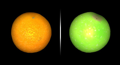
Fig 1.1: Screen captures of orange and apple shaders

For an OpenGL project I am helping fellow NYU-ITP graduate student Matt Parker with; I developed two real-time shaders written in GLSL to be applied to poly-spheres representing two types of fruit: apples and oranges. Due to the sheer number of spheres being displayed, the object on my end was to get a high-amount of surface detail using a limited amount of polygons. To accomplish this, I used a combination of displacement and normal mapping calculation in the shader, meaning that all surface detail is accomplished through the GPU.

I have already written about how displacement is done through shaders - the very same technique I used in the past was also used in this set of shaders:
Geometry Displacement through GLSL

Color variance along the geometric surface in regard to light has changed apart from my past shader work, where I have written in ambient and specular calculations through accessing the light (L) and given surface material (M), where:

Diffuse:


Ambient:


Specular (where H is the given half-vector):


To simulate the surface shape variance needed to pull off the appearance of an orange, a popular technique called "bump-mapping" was used. Bump-mapping is generally accomplished by having a normal-map which is sampled as XYZ vectors which are supplemented across the geo-normal matrix that the shader is applied to. The Lambert term for the normal is calcuated, which is simply the dot product of the normal and the light direction. If the lambert term is above 0.0, calcuate specular and add to the final color for the fragment. Here is some sample code to illustrate:

vec3 N = texture2D(normalMap, gl_TexCoord[0].st).rgb *
               2.0 - 1.0;
float lambert_term = max(dot(N,L),0.0);

if (lambert_term > 0.0)    {
// Compute specular
vec3 E = normalize(eyeVec);
vec3 R = reflect(-L, N);
float specular = pow(max(dot(R, E), 0.0),
                     gl_FrontMaterial.shininess);
}

The finished shader encompasses texturing, displacement, and normal mapping, resulting in a nice aesthetic simulating a complex surface with light calculations matching the surface variance. All of this occurring on a low-poly (16 x 16) quadric sphere object. Rotation animation simulated in real-time of the orange shader below:


Fig 1.2: Orange shader rotation animation


Sources for general information/reference and equation images:
ozone3D.net
Lighthouse3D.com
OpenGL.org

Maya: Fluid Gradient Programming (Plug-In)

Fig 1.1: Still of fluid-based fire simulation, with colors generated through plug-in gradient mapping system

I am currently developing a plug-in for Maya, a popular 3D modeling/animation package. The goal for the plug-in as a whole is to reinvent how fluid dynamic systems/effects are developed in Maya by constructing a node-based GUI which can be used within Maya, with each node encapsulating a current feature Maya fluids currently have - essentially adding on a layer of abstraction for the user to more easily generate simulations. The plug-in also aims to extend the current feature set of fluids within Maya.

I decided to start the development of the plug-in with a quick experiment, that being the integration of the generic gradient object class I developed earlier this semester with the Maya native gradient data driving color and incandescence. The aim being that images could be sampled and have their most dominate colors applied to the color/incandescence of the fluid voxel-system within Maya - thus automating the construction of the color palette for a given effect. The results and rendered video are posted below:


Fig 1.2: Default Maya Fluid Effects values



Fig 1.3: Early development of Maya plug-in as a drop-menu



Fig 1.4: Image chosen to have dominate colors sampled



Fig 1.5: Image sampled gradient constructed and mapped into Maya's attribute data



Fig 1.6: Fluid fire simulation animation, colors derived from gradient sampling without modification

Animation: Luma-Displacement / Glow (OpenGL / GLSL)

Sphere with an animated displacement GLSL shader that calculates a glow / bloom effect along defined distance from midpoint.

Luma-Based Displacement

Fig 1.1: In-progress glacier shader with geometric displacement

Python vs. Java vs. Python/Weave

In case you haven't noticed, I am a rather big proponent of using Python whenever possible. Between Python's flexibility and just the enjoyment I get out of writing in the language, I generally look to use Python before turning to a static language such as C/C++ or Java. The times I have had to turn to a compiled language are usually linked to when I need computational speed.

There are several ways to get Python moving faster - some a bit more ugly than others; code speedups with Python are usually about trading in readability for performance, but that doesn't mean it can't be straight-forward in implementation. In the past, I have used the usual bag of Python tricks: list comprehensions, method/variable assignment outside loops, generators, and countless more pure-Python solutions.

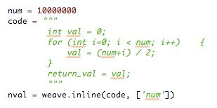
Recently, I stumbled upon Weave, a module existing inside the popular SciPy library which allows for C code to be mixed with Python code. Using Weave allows for the coder to stay inside the bounds of Python, yet use to power of C to compute the heavier algorithms. Not only does it provide a speed increase... it beats Java. Consider this (nonsensical) algorithm comparison between pure Python, Java, and Weave + Python:


Python Example:

Time: 1.681 sec.


Java Example:

Time: 0.037 sec.


Python + Weave Example:

Time: 0.017 sec.


Using identical algorithms in all three tests; using Weave with Python was nearly 100 times faster (98.9x) than using pure Python alone. In comparison to Java, Weave + Python was a shade over 2 times faster (2.1x) than Java. Although the Python/Weave code itself is bigger than the pure Python and Java examples - the speed it provides is absolutely phenomenal, without ever leaving your .py file.

Hopefully, I'll be able to use the power of mixing C with Python for more elaborate purposes - but this test alone is enough to get me excited about future projects with Python.

DayBRIGHT: Gradient / Render Integration

I have now managed to get DayBRIGHT to render out a full animation using a gradient as the light source. While the animation scene itself is rather basic, with three spheres inside a box, it demonstrates some of the primary goals of the project.

Now that the gradient data structure integrates with the rendering process, it now becomes a matter of writing the translators for each type of media I'd like to use - as well as developing a more interesting scene to light.




Fig 1.1 + 1.2: Animation using displayed gradient as lighting source over time


Indirect surface shader code:

DayBRIGHT: Post-Processing

Changing gears a bit, I decided to begin writing in some post-image processing functionality to DayBRIGHT to handle the final image output. The first post-process was writing a color noise filter that blended a 1:1 ratio of random colored pixels with each rendered image . This is done to counter the fact that the illusion of computer graphics being reality is often blown due to a discrepancy in noise artifacts across the image, most commonly noticed when graphics are composited with film or video footage. Even without footage, the human mind does not normally process perfectly smooth color and shape with reality. Reality rarely has instances of complete visual fidelity, at least from an everyday human perspective.


Fig 1.1: Simple color noise composite process

Another post-process that is necessary was gamma correction. The algorithm resulting from the equation is straight-forward, where a gamma corrected set of values from 0-255 is created, then each RGB value from the given image is changed to the gamma corrected equivalent. Below is the simple math equation for gamma correction and corresponding algorithm in (non-optimized) Python code:


Fig 1.2: Gamma correction equation

DayBRIGHT: Renderman Rendering

Below are some test renders coded through Renderman and woven into the DayBRIGHT graphics and data handling subsystems. Using the classic Cornell box, I was able to successfully simulate global illumination in combination with image based lighting. The photon calculation isn't as smooth (or as fast) as I'd like it to be - but optimization will be taken care of later once I can generate reliable image sequences.


Fig 1.1: Global illumination / color bleeding


Fig 1.2: Image-based lighting with accurate shadows. Shadows no longer gradient of grays, but rather mixed with color pertaining to casting objects.


Fig 1.3: Classic Cornell box setup with pronounced color bleed

DayBRIGHT: Image to Gradient Translation

The first translator I decided to fully flesh out for DayBRIGHT is the static image translator. The underlying system I have developed only has one principle rule - anything can be translated and used, as long as that translation returns a gradient object. So, how can a gradient be created from an image?

I took the route of writing an algorithm which finds and stores the most dominate colors in an image - then using each sample as a control point within a varying length linearly-smoothed gradient, where the most dominate colors are in order from left to right. Below are some examples of the results, where the top is the source that was sampled and gradient is the output visualized:


Fig 1.1: Sky converted to a gradient based on dominate colors


Fig 1.2: Composition VI, W. Kandinsky - image to gradient conversion


Fig 1.3: Composition VII, W. Kandinsky - image to gradient conversion

Now that a method existed to translate static images into gradients, it becomes a trivial task to write a translator for a video feed, as video can be easily treated as a series of images. Simple alterations to a subsystem can allow for a calculated sample of each frame in a gradient. So, if a video feed were parsed once every hour for twenty four hours, a gradient could be constructed of n-length, linearly being smoothed evenly across each respective control point based on n+1 distance.

DayBRIGHT: Generic Structures

The underlying system DayBRIGHT uses to translate various data structures has become less about constraining data to a set format, and more about developing a generic structure (a gradient) to fully represent the data in an elegant way. I find this an interesting topic to explore because it has really opened a lot of doors as to how far I can take his project; in particular, in the sheer variance of data I can now use.

RSS feeds, video streams, static images, audio tracks, physical sensor data - all of which can be harbored by a single generic data structure. Each piece of data simply needs its own translator towards being converted to the structure; once that is done - there is no further special-casing needed.

My goal for this project is to have, by the end of semester, a demonstration of how the various types of data listed above can be used to achieve results for an identical operation. In the case of DayBRIGHT, I will be using the gradient structures to light 3D geometry. How this will be done merits its own detailed entry - which is forthcoming.

I am really excited about this idea, it is a blend of engineering/mathematics and visual aesthetics that I have always been drawn to. I am dedicating all of my classes to it in hope that my time commitment will really push this idea as far as it can go.